Part 2: Computer Vision @ GIPHY: How we Created an AutoTagging Model Using Deep Learning
January 11, 2021 by

This is part two of the GIPHY Autotagging blog post series, where we’ll cover modeling, configuration of our training environment, and share our results. In part one, we outlined our motivation for this product and provided an overview of existing related approaches. Additionally, we described the training and evaluation data we have at hand and our custom methodology for filtering and enrichment.
If you haven’t read part one, you should check it out (here) before reading this post.
Our Training Environment
For this project, we conducted all our experiments on Amazon Sagemaker, and primarily relied on architectures written in PyTorch because of its simplicity, convenience for prototyping, and optimization features. All the code was written using this framework.
To ensure reproducibility and full control over different experiments, we leveraged the Catalyst framework, which allows us to structure PyTorch experiments in a clean and concise way, enabling engineers to omit rewriting the same training loop every time. Furthermore, Catalyst provides an intuitive high-level interface over extremely handy PyTorch tools we benefited from:
- Distributed Data Parallel – distributed mode for PyTorch, allow use of multiple GPU devices
- Apex – PyTorch extension with NVIDIA utilities for mixed precision and distributed training
- Torch JIT – modern way to serialize and optimize PyTorch models for inference
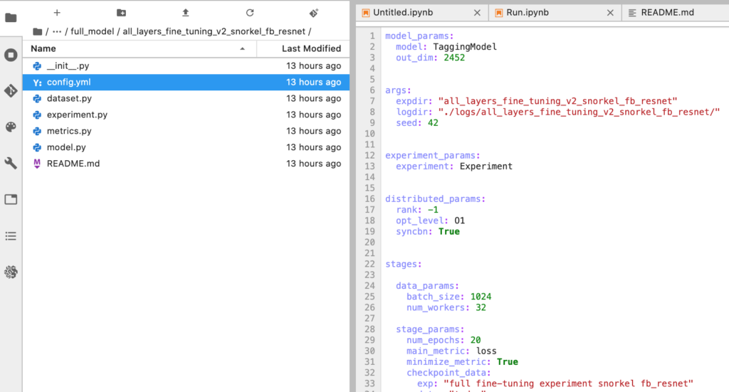
As you can see, components for training need to be defined in separate files: model, dataset, custom metrics (if any) etc. Afterwards, they can be organized into a training pipeline via config.yml file. To start a corresponding experiment we can use catalyst-dl command-line tool like this:
catalyst-dl run -config=all_layers_fine_tuning_v2_snorkel_fb_resnet/config.yml --verbose
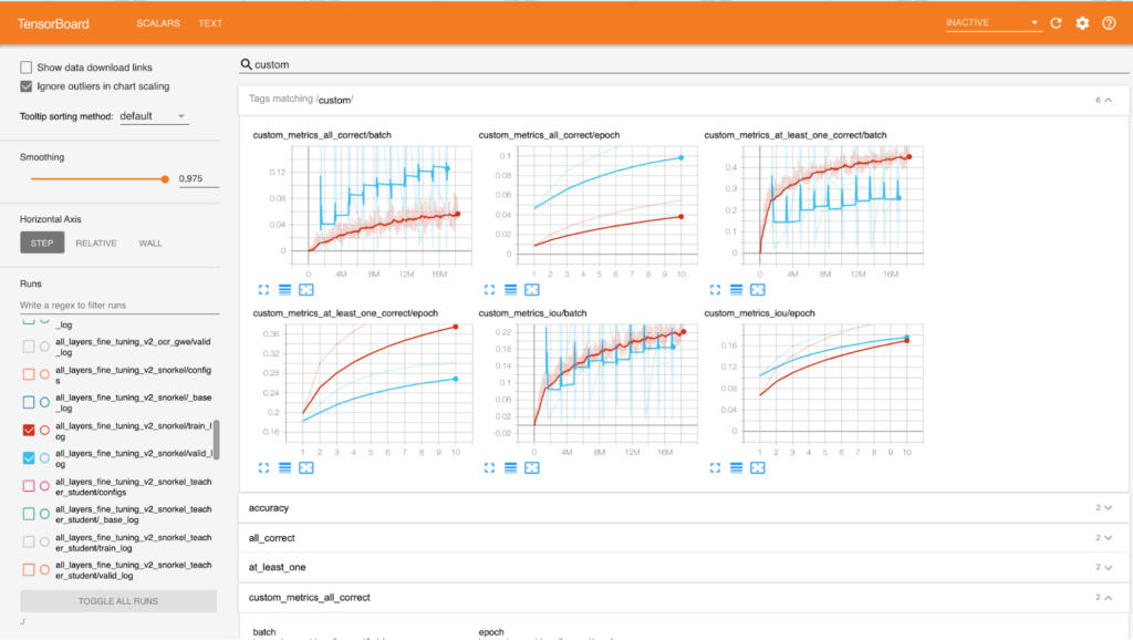
This command will launch the training routine and record actual code that was executed with all dependencies, checkpoints, and metrics in TensorBoard format.
Training and Evaluation
As mentioned previously, we decided to consider this task as a multilabel classification, therefore, model outputs sigmoids and Binary Cross Entropy Loss are used as a main criterion. For the learning rate policy we picked Cyclic Learning Rate and Adam for the optimizer — training tools which have worked best for us in the recent Computer Vision projects. A majority of our experiments were done using the ResNext101 model from FB WSL research. Additionally, we came up with the following list of metrics to evaluate our training progress:
IOU (Intersection Over Union)
For each GIF we take its actual tags (say, N tags) and take top N classes from the model’s output (sigmoids). IOU is an intersection between actual tags and those top N predicted tags (value from 0 to 1) normalized by the size of their union. To aggregate this metric for the batch, we simply compute the mean value of all these intersections.
“At-Least-One-Correct”
This metric is similar to IOU, but instead of the actual intersection value we calculate the percentage of GIFs from the batch for which IOU is not zero (value from 0 to 1).
“All-Correct“
This metric is also based on the intersection described above, but here we count GIFs with 100% IOU between actual and predicted tags (value from 0 to 1).
Semantic Accuracy
As observed within our experiments, aforementioned metrics values are not as high as we would expect. This can be explained by generalization capabilities of the model: for example, when a GIF depicts a soccer scene and actual tags are “soccer“ and “goal,“ but our model predicts “soccer“ and “ball.“ IOU value for this case is 0.5, which doesn’t reflect that overall the tags are pretty relevant. It means that exact matching results in lower metrics than we subjectively perceive. To tackle this problem we came up with a metric which estimates similarity between actual and predicted tags in the latent semantic vectors space. For this purpose we used an internal semantic model called Tag2Vec that provides meaningful embeddings for tags. We simply map labeled and predicted tags onto this embedding space, compute pairwise cosine distances, and find minmax distance value for the final metric.
Experiments
Head Fine-Tuning
We started with a simple idea: remove the last fully-connected layer of pre-trained ResNext101 model and replace it with our fully-connected layer to map latent vectors onto a set of our tags (not Imagenet labels). Only this new layer is trained — the CNN is frozen. After that, we added more fully-connected layers with RELU activations and batch norms, but it didn’t result in significant improvements.
Full Fine-Tuning
To go further, we unfreeze all layers in the neural network including convolutional blocks. This change brought the model to a completely new quality level — metrics went up more than 3%. You can see some of predictions made by our model below:

Comparison of Facebook WSL ResNet vs Torchvision Imagenet Resnet
Since the FB WSL models were fine-tuned on Imagenet, the natural question would be: “why do we use a FB WSL model instead of a more common model, pre-trained on Imagenet, taken from torchvision package?“ To address this concern, we repeated the previous experiment for Imagenet pre-trained ResNet50 model from torchvision and compared it to the ResNet50 WSL model we fine-tuned.
What we observed is that FB WSL outperforms a pure Imagenet pre-trained model. Therefore, it seems that representations of the FB WSL model are easier to fine-tune on a GIPHY dataset than a plain Imagenet model.
Semi-supervised learning
Looking at the results of the previous experiments, we have an assumption that the low performance of the model is related to the noisy training dataset. To verify this, we cleaned our dataset with predictions of our SOTA model by taking the following steps:
- We take original labels and predictions (sigmoids) from the model for the given training sample
- If the original label is available in prediction with confidence value bigger than some threshold value, we leave it unchanged
- Otherwise, the score assigned to the original label is reduced by half
- All predicted labels with confidence ≥ another threshold value are added to the sample (if not present already) with corresponding score
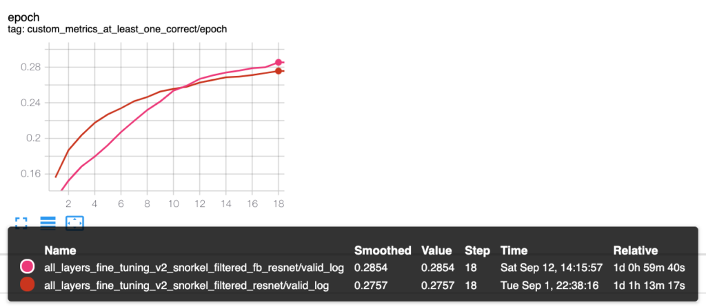
By doing this, we both filter out unconfident labels and generate new ones by using our current best model. We trained a new model on this updated dataset. This strategy allowed us to improve our metrics a bit (approximately 1% improvement of IOU).
Teacher-Student learning
Since our final goal is to serve this model’s predictions to actual GIPHY users, addressing performance concerns is critical to delivering the best experience to our users. So far, we’d primarily utilized a huge FB WSL model — ResNext101, which inference time on a CPU instance is around 1 second (c5.4xlarge ec2 instance, 16 cores, 32GB of RAM).
Therefore, we thought we might follow a modern knowledge distillation approach to get the most out of our SOTA model and transfer its behaviour to a more lightweight model — ResNet50 (also from WSL research) which has much better timing (~200 ms on the same c5.4xlarge instance) and size (approximately 3 times smaller than ResNext101 in terms of parameters number). Our assumption was, this new model’s quality should be on par with a large WSL model.
Hereafter, in this section we reference ResNext101 as “Teacher model” and ResNet50 as “Student model.” To train the Student model we used a multi-task loss that is calculated as a weighted sum of two components:
- Loss based on original labels for the sample
- Loss based on predictions (sigmoids) of Teacher model for the same sample
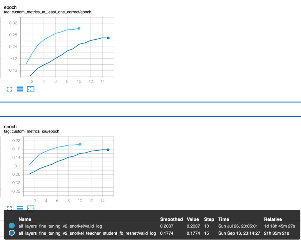
As it turned out, the Student model performs considerably worse (by 2-3%) according to all metrics. This can also be seen when the model is tested manually. What’s even more interesting, when any component is removed from our combined loss (labels or predictions) it doesn’t affect the metrics. The same effect can be observed when the Student is trained on the original labels only. We can’t sacrifice such a considerable precision gap for the sake of performance, but we’re actively investigating ways to optimize inference speed through various compression techniques.
Deployment
To serve the AutoTagging model in the production environment we export it via PyTorch JIT. This has multiple benefits, such as compact serialized checkpoint and ability to load and use a model without having an actual model definition in code.
To wrap the model into a real-time service we use the Seldon framework. It automatically generates both REST and GRPC services given only a Python class where behaviour of your model is defined. Apart from that, these services are already instrumented in collecting metrics that can be easily exported to Prometheus, Jaeger etc. Also, Seldon provides out-of-the-box ability to run A/B tests to compare different models. Our Seldon environment is running in a Kubernetes cluster and we leverage GPU powered instances for faster inference.
The first user-facing interface on the GIPHY platform to integrate the AutoTagging model is the “GIF Edit” modal, which is a popup allowing users to edit one of their uploaded GIFs. As it can seen in the example below, a user is provided with a set of tags suggested by the model.
If a GIF doesn’t have tags, all the suggestions come from our AutoTagging model. If there are pre-existing tags on the GIF, we supplement Autotagging Model suggestions with suggestions from a custom NLP model which are semantically similar to the pre-existing tags. To track performance, we track “seen,” “add,” and “reject” events for all tags so we know which tags a user finds appropriate or irrelevant. This data will be used to improve the model over time.
We did a preliminary analysis of this feature’s impact on the newly added content for the last month. As a result, we report that following the launch for some of the verified users cohorts:
- Percentage of uploaded GIFs without tags dropped down by 45%
- Percentage of uploaded GIFs with one tag dropped by more than 13%
- Percentage of uploaded GIFs with multiple tags increased by 2%
- Average number of tags per uploaded GIF increased by almost 39%
Even by looking at these simple metrics we can clearly see a positive trend after the model was released. What these numbers basically mean is that new content will be handled more effectively by our search engine and bring more fun to our users. Furthermore, this is just the first iteration of the AutoTagging project and we’ll keep on iterating on both model and UI/UX to provide an even better experience.
Creating this AutoTagging model was one of the most challenging and rewarding projects our team has ever worked on, and we’re extremely proud of our results and excited to keep iterating on this model. We hope you found this article helpful, and perhaps it can provide guidance to anyone else working on a similar project. Please reach out to us on Twitter with any questions or comments.
— Dmitry Voitekh, AutoTagging tech lead
Additionally, many thanks to Proxet and their engineers for their valuable contributions to the project!
GIPHY Engineering Signals Team
— Nick Hasty
— Dmitry Voitekh
— Ihor Kroosh
— Taras Schevchenko
— Vlad Rudenko