Beyond Content: Extracting Image Property Data from GIFs
October 24, 2017 by
For my summer internship on the GIPHY engineering team, I was tasked with extracting image property data from GIFs. Image property data is metadata about the GIF files themselves, particularly attributes that affect human perception and image “quality”, as opposed to content-related metadata.
GIPHY can then use this data to do things like build predictive models that can help categorize and label GIFs, find correlations with other data points like popularity, optimize file generation and generally learn more about the overall makeup of their massive GIF catalog,
Here is a list of some of the properties we settled on:
Transparency: GIF pixels are encoded with the RGBA color space format where RGBA stands for Red, Green, Blue, and Alpha. The color is encoded in the first 3 values (with integers between 0 and 255) and the last value corresponds to a transparency element and is either 0 (transparent) or 255 (not-transparent). We use transparency percentage to distinguish between Stickers and regular GIFs, and though we already compute overall transparency, we supplemented this existing data by also computing the ratio of pixels that are transparent for every frame and then computing the mean, the standard deviation and the skewness of this ratio.
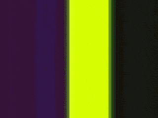
Brightness: Brightness (aka Value as in HSV) measures the degree to which something appears to be radiating or reflecting light. We calculate the brightness of each pixel of each frame by converting RGB to HSV, and these values are then averaged in order to get one single value for each frame. We compute the mean, standard deviation and skewness of the brightness over all a GIF’s frames.
A GIF with high brightness:
A GIF with low brightness:
Luminosity: Luminosity (aka Lightness) measures how we perceive a color’s brightness, or the amount of white in the color, and is also known as tone. We calculate the lightness of each pixel of each frame by converting RGB to HSL, and these values are then averaged in order to get one single value for each frame. We compute the mean, standard deviation and skewness of the lightness over all a GIF’s frames.
Both of these GIFs have “bright” color tones and thus high luminosity:
Contrast: Contrast is the difference in luminance or color that makes an object distinguishable. It can be computed by taking the square root of the distance between an individual frame’s lightness and the GIF’s overall lightness. We compute the mean, standard deviation and skewness of the contrast over all a GIF’s frames.
A high contrast gif, frame colors and brightness change dramatically for the duration of the gif:
A very low contrast gif, it’s hetergenous in color and brightness for the duration of the gif:
Sharpness: Perceived sharpness is a measure of image resolution and “acutance”, and describes how we perceive the contrasts in edges and boundaries between items in an image. Sharp images have clearly delineated details, while in blurry image it’s difficult to distinguish objects and boundaries. To get sharpness, we compute the average gradient magnitude for each frame. We then compute the mean, standard deviation and skewness over all frames. We also compute an histogram of the values.
This GIF has high sharpness due to high resolution textures and patterns:
This GIF has low sharpness due to lack of color variation and the blurriness between objects:
Entropy: Image entropy describes the amount of information in an image; it’s a measurement of the number of “states” contained within the image, or how “busy” it is. We compute the entropy of each frame of a GIF by calculating the probability of difference between adjacent pixels. A high probability means high entropy, and low probability means low entropy. We then compute the mean, standard deviation and skewness over all frames.
This GIF from the Simpsons intro has high entropy due to the wide variety of characters and objects it:
This GIF has low entropy because the minimal amount of movement and color results in a small difference in pixel values:
Noise: Noise is unintentional distortion, like random fluctuations in brightness and color, that reduces the visibility or quality of an image. We compute noise in two ways. First apply a median filter on a frame, and then compute the MSE distance between the original frame and the filtered one. Second, we use total variation denoising to create a denoised version of the original and compute SSIM and PSNR distance between the frames. For both, we compute the mean, standard deviation and skewness over all frames.
Example of a noisy GIF:
For this GIF, the average SSIM difference across frames of the original noisy frames (example frame left) and the total variation denoised frames (example right) is .33/1.00, indicating the original is a very noisy gif.
Motion: This property represents the overall motion energy in a GIF, and is calculated from a GIF’s Motion History Image (MHI). The MHI is a grayscale transformed image that uses black, white and shades of gray to capture motion history. In the example below, the rightmost image is the MHI of a GIF. The black area corresponds to the part where there is no movement, the white area to the recent movement and the gray one to the old movement. We compute the histogram over the different grayscale colors of the MHI in order to get the area of each of these colors in the MHI.
The motion histogram created from the above GIF:
Color Histogram: We wanted to find the 10 dominant colors in a GIF and the percentage of pixels for these displaying colors. After experimenting with K-means clustering, we found a faster method with equal if not better results. The idea behind it is to get a binary tree of colors that are in the image and to do the separation between two “close” colors based on the two colors that have the biggest eigenvalues in it covariance matrix. Furthermore, as each frame could use a different palette of colors, and as I wanted to get 10 colors for the whole GIF, I had to first concatenate all the frames inside one image and then apply this method. The results of this method are very good as it enables to get very different colors and their pixel proportion with a decent running time.
Loopiness: A metric specifically for GIFs, we wanted some way to measure a GIF’s “loopiness”, that is how perfectly the ending of GIF syncs up with it’s beginning. After a number of experiments, we ended up doing distance comparisons between a percentage of frames in the beginning and ending of the GIF, eg the 1st frame and the last frame, the 2nd frame and the penultimate frame, and so on. We also added a “continuous loopiness” algorithm that performs the same operation but against all adjacent frames. For these algorithms, we ended up using 4 distance metrics: MSE (Mean Square Error), NRMSE (Normalized Root Mean Square Error), PSNR (Peak Signal-to-Noise Ratio), SSIM (Structural Similarity), and we estimate “loopiness” based on the mean of those values per frame. As documented, the SSIM comparison seem to be the most indicative of similarity.
GIFs with high “loopiness” values:
GIPHY is now in the process of computing these properties and other metrics against tens of millions of GIFs. A number of investigations and experiments are planned, so stay tuned to the GIPHY Engineering blog for updates on their progress.
– Ruben Stern, Engineering Intern